Logistic-Regression 실습

분류 모델 실습

pima-indians-diabetes.csv 파일을 읽어서, 당뇨병을 분류하는 모델을 만드시오.

컬럼 정보 :

Preg=no. of pregnancy

Plas=Plasma

Pres=blood pressure

skin=skin thickness

test=insulin test

mass=body mass

pedi=diabetes pedigree function

age=age

class=target(diabetes of not, 1:diabetic, 0:not diabetic)

import numpy as np
import pandas as pd
import matplotlib.pyplot as plt
import seaborn as sb

%matplotlib inline

import platform

from matplotlib import font_manager, rc
plt.rcParams['axes.unicode_minus'] = False

if platform.system() == 'Darwin':
    rc('font', family='AppleGothic')
elif platform.system() == 'Windows':
    path = "c:/Windows/Fonts/malgun.ttf"
    font_name = font_manager.FontProperties(fname=path).get_name()
    rc('font', family=font_name)
else:
    print('Unknown system... sorry~~~~')

df = pd.read_csv('pima-indians-diabetes.csv')

df

	Preg	Plas	Pres	skin	test	mass	pedi	age	class
0	6	148	72	35	0	33.6	0.627	50	1
1	1	85	66	29	0	26.6	0.351	31	0
2	8	183	64	0	0	23.3	0.672	32	1
3	1	89	66	23	94	28.1	0.167	21	0
4	0	137	40	35	168	43.1	2.288	33	1
...	...	...	...	...	...	...	...	...	...
763	10	101	76	48	180	32.9	0.171	63	0
764	2	122	70	27	0	36.8	0.340	27	0
765	5	121	72	23	112	26.2	0.245	30	0
766	1	126	60	0	0	30.1	0.349	47	1
767	1	93	70	31	0	30.4	0.315	23	0

768 rows × 9 columns

df.isna().sum()

Preg     0
Plas     0
Pres     0
skin     0
test     0
mass     0
pedi     0
age      0
class    0
dtype: int64

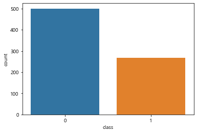
sb.countplot(data=df,x='class')
plt.show()

X = df.iloc[:,:8]

y= df['class']

# preg 컬럼은 0이 들어가도 된다.
# 이 컬럼을 제외한 나머지 컬럼들에 0이 있으면 모두 np.nan으로 변경

X.iloc[:,1:] = X.iloc[:,1:].replace(0,np.nan)

X.describe()

	Preg	Plas	Pres	skin	test	mass	pedi	age
count	768.000000	763.000000	733.000000	541.000000	394.000000	757.000000	768.000000	768.000000
mean	3.845052	121.686763	72.405184	29.153420	155.548223	32.457464	0.471876	33.240885
std	3.369578	30.535641	12.382158	10.476982	118.775855	6.924988	0.331329	11.760232
min	0.000000	44.000000	24.000000	7.000000	14.000000	18.200000	0.078000	21.000000
25%	1.000000	99.000000	64.000000	22.000000	76.250000	27.500000	0.243750	24.000000
50%	3.000000	117.000000	72.000000	29.000000	125.000000	32.300000	0.372500	29.000000
75%	6.000000	141.000000	80.000000	36.000000	190.000000	36.600000	0.626250	41.000000
max	17.000000	199.000000	122.000000	99.000000	846.000000	67.100000	2.420000	81.000000

X.isna().sum()

Preg      0
Plas      5
Pres     35
skin    227
test    374
mass     11
pedi      0
age       0
dtype: int64

# 현재 X 와 y로 분리한 상태에서 0을 NaN으로 바꿨다.
# 따라서 Nan을 삭제할 경우! y 도 함께 처리해줘야 하는데, 어렵다.
# 그러므로 NaN 을 삭제하고 싶으면, X와 y 분리 전에 해줘야 한다.
# 이 예에서는, Nan을 각 컬럼의 평균값으로 채우는 전략을 사용한다.
X = X.fillna(X.mean())

X.isna().sum()

Preg    0
Plas    0
Pres    0
skin    0
test    0
mass    0
pedi    0
age     0
dtype: int64

from sklearn.preprocessing import StandardScaler

scaler = StandardScaler()

X = scaler.fit_transform(X)

# 학습용 데이터와 테스트용 데이터.

from sklearn.model_selection import train_test_split

X_train,X_test,y_train,y_test = train_test_split(X,y,test_size = 0.2,random_state= 10)

from sklearn.linear_model import LogisticRegression

classifier = LogisticRegression(random_state=10)

classifier.fit(X_train,y_train)

LogisticRegression(random_state=10)

y_pred = classifier.predict(X_test)

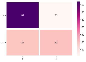
from sklearn.metrics import confusion_matrix

cm=confusion_matrix(y_test,y_pred)
cm

array([[84, 11],
       [29, 30]], dtype=int64)

from sklearn.metrics import classification_report

print(classification_report(y_test,y_pred))

              precision    recall  f1-score   support

           0       0.74      0.88      0.81        95
           1       0.73      0.51      0.60        59

    accuracy                           0.74       154
   macro avg       0.74      0.70      0.70       154
weighted avg       0.74      0.74      0.73       154

# 컨퓨전 메트릭스를, 히트맵으로 그려서 보기

sb.heatmap(data=cm,annot=True, cmap='RdPu',linewidths=5)
plt.show()