Prophet을 이용한 가격예측 -colab
AVOCADO 가격 예측 (Facebook Prophet )
STEP #0: 데이터셋
- 데이터는 미국의 아보카도 리테일 데이터 입니다. (2018년도 weekly 데이터)
- 아보카도 거래량과 가격이 나와 있습니다.
컬럼 설명 :
- Date - The date of the observation
- AveragePrice - the average price of a single avocado
- type - conventional or organic
- year - the year
- Region - the city or region of the observation
- Total Volume - Total number of avocados sold
- 4046 - Total number of avocados with PLU 4046 sold - PLU는 농산물 코드입니다
- 4225 - Total number of avocados with PLU 4225 sold
- 4770 - Total number of avocados with PLU 4770 sold
STEP #1: 데이터 준비
Prophet 라이브러리
-
install : pip install fbprophet
-
위 에러 발생시 : conda install -c conda-forge fbprophet
-
레퍼런스 : https://research.fb.com/prophet-forecasting-at-scale/ https://facebook.github.io/prophet/docs/quick_start.html#python-api
# import libraries
import pandas as pd
import numpy as np
import matplotlib.pyplot as plt
import random
import seaborn as sns
from fbprophet import Prophet
from google.colab import drive
drive.mount('/content/drive')
Mounted at /content/drive
import os
os.chdir('/content/drive/MyDrive/python/day15')
# avocado.csv 데이터 읽기
avocado_df = pd.read_csv('avocado.csv',index_col=0)
STEP #2: EDA(Exploratory Data Analysis) : 탐색적 데이터 분석
avocado_df
| Date | AveragePrice | Total Volume | 4046 | 4225 | 4770 | Total Bags | Small Bags | Large Bags | XLarge Bags | type | year | region | |
|---|---|---|---|---|---|---|---|---|---|---|---|---|---|
| 0 | 2015-12-27 | 1.33 | 64236.62 | 1036.74 | 54454.85 | 48.16 | 8696.87 | 8603.62 | 93.25 | 0.0 | conventional | 2015 | Albany |
| 1 | 2015-12-20 | 1.35 | 54876.98 | 674.28 | 44638.81 | 58.33 | 9505.56 | 9408.07 | 97.49 | 0.0 | conventional | 2015 | Albany |
| 2 | 2015-12-13 | 0.93 | 118220.22 | 794.70 | 109149.67 | 130.50 | 8145.35 | 8042.21 | 103.14 | 0.0 | conventional | 2015 | Albany |
| 3 | 2015-12-06 | 1.08 | 78992.15 | 1132.00 | 71976.41 | 72.58 | 5811.16 | 5677.40 | 133.76 | 0.0 | conventional | 2015 | Albany |
| 4 | 2015-11-29 | 1.28 | 51039.60 | 941.48 | 43838.39 | 75.78 | 6183.95 | 5986.26 | 197.69 | 0.0 | conventional | 2015 | Albany |
| ... | ... | ... | ... | ... | ... | ... | ... | ... | ... | ... | ... | ... | ... |
| 7 | 2018-02-04 | 1.63 | 17074.83 | 2046.96 | 1529.20 | 0.00 | 13498.67 | 13066.82 | 431.85 | 0.0 | organic | 2018 | WestTexNewMexico |
| 8 | 2018-01-28 | 1.71 | 13888.04 | 1191.70 | 3431.50 | 0.00 | 9264.84 | 8940.04 | 324.80 | 0.0 | organic | 2018 | WestTexNewMexico |
| 9 | 2018-01-21 | 1.87 | 13766.76 | 1191.92 | 2452.79 | 727.94 | 9394.11 | 9351.80 | 42.31 | 0.0 | organic | 2018 | WestTexNewMexico |
| 10 | 2018-01-14 | 1.93 | 16205.22 | 1527.63 | 2981.04 | 727.01 | 10969.54 | 10919.54 | 50.00 | 0.0 | organic | 2018 | WestTexNewMexico |
| 11 | 2018-01-07 | 1.62 | 17489.58 | 2894.77 | 2356.13 | 224.53 | 12014.15 | 11988.14 | 26.01 | 0.0 | organic | 2018 | WestTexNewMexico |
18249 rows × 13 columns
데이터의 날짜가 뒤죽박죽 입니다. 날짜로 정렬하시오.
avocado_df = avocado_df.sort_values('Date')
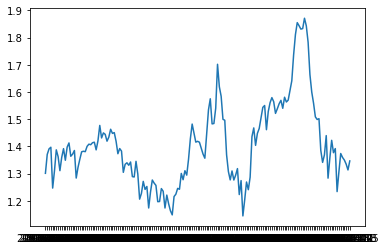
날짜별로 가격이 어떻게 변하는지 간단하게 확인하시오. (plot 이용)
df_date = avocado_df.groupby('Date')['AveragePrice'].mean()
plt.plot(df_date)
plt.show()
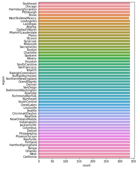
‘region’ 별로 데이터 몇개인지 시각화 하시오.
plt.figure(figsize=(6,10))
sns.countplot(data= avocado_df,y = 'region')
plt.show()
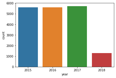
년도(‘year’)별로 데이터가 몇건인지 확인하시오.
sns.countplot(data= avocado_df,x='year')
plt.show()
프로펫 분석을 위해, 두개의 컬럼만 가져오시오. (‘Date’, ‘AveragePrice’)
avocado_prophet_df = avocado_df[['Date','AveragePrice']]
avocado_prophet_df
| Date | AveragePrice | |
|---|---|---|
| 51 | 2015-01-04 | 1.75 |
| 51 | 2015-01-04 | 1.49 |
| 51 | 2015-01-04 | 1.68 |
| 51 | 2015-01-04 | 1.52 |
| 51 | 2015-01-04 | 1.64 |
| ... | ... | ... |
| 0 | 2018-03-25 | 1.36 |
| 0 | 2018-03-25 | 0.70 |
| 0 | 2018-03-25 | 1.42 |
| 0 | 2018-03-25 | 1.70 |
| 0 | 2018-03-25 | 1.34 |
18249 rows × 2 columns
STEP 3: Prophet 을 이용한 예측 수행
ds 와 y 로 컬럼명을 셋팅하시오.
# 날짜 컬럼은 ds로 예측하고자 하는 가격 컬럼은 y로 바꿔준다.
avocado_prophet_df = avocado_prophet_df.rename(columns={'Date':'ds','AveragePrice':'y'})
avocado_prophet_df
| ds | y | |
|---|---|---|
| 51 | 2015-01-04 | 1.75 |
| 51 | 2015-01-04 | 1.49 |
| 51 | 2015-01-04 | 1.68 |
| 51 | 2015-01-04 | 1.52 |
| 51 | 2015-01-04 | 1.64 |
| ... | ... | ... |
| 0 | 2018-03-25 | 1.36 |
| 0 | 2018-03-25 | 0.70 |
| 0 | 2018-03-25 | 1.42 |
| 0 | 2018-03-25 | 1.70 |
| 0 | 2018-03-25 | 1.34 |
18249 rows × 2 columns
프로펫 예측 하시오.
# 변수로 만들기
prophet = Prophet()
# 2. 기존의 날짜와 데이터로 학습시키기
prophet.fit(avocado_prophet_df)
INFO:numexpr.utils:NumExpr defaulting to 2 threads.
INFO:fbprophet:Disabling weekly seasonality. Run prophet with weekly_seasonality=True to override this.
INFO:fbprophet:Disabling daily seasonality. Run prophet with daily_seasonality=True to override this.


<fbprophet.forecaster.Prophet at 0x7f0fb48b1250>
# 365일치를 예측하시오.

# 3. 예측하고자 하는 기간을 정해서, 기간만 나와있는 데이터 프레임 만들기
future = prophet.make_future_dataframe(periods=365)
# 4. 프로펫의 predict 함수를 이용해서, 실제로 예측한다.
forecast = prophet.predict(future)
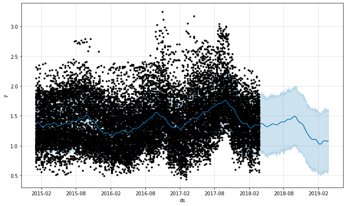
# Time Series(타임 시리즈) 데이터.
# 차트로 확인하시오.
prophet.plot(forecast)
plt.savefig('chart1.jpg') # 코랩과 버그가 있어 차트가 2개씩 뜨므로 하나는 저장하여 안보이게 할 수 있다.
prophet.plot_components(forecast)
plt.savefig('chart2.jpg')
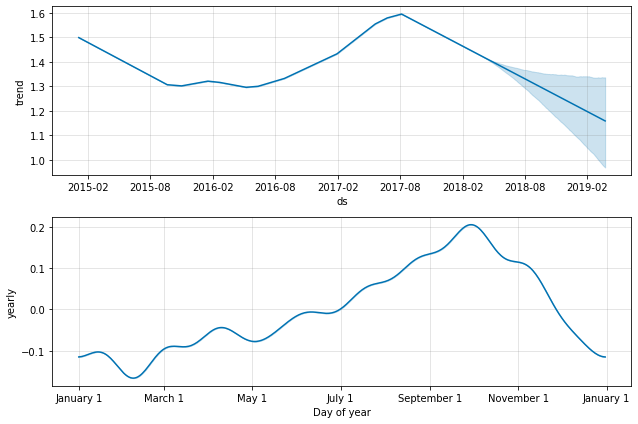
# trend 는 앞으로의 방향성 위,아래로는 상한선과 하한선을 의미
# yearly 는 주기성을 의미한다.
PART 2 : region 이 west 인 아보카도의 가격을 예측하시오.
west_df = avocado_df.loc[avocado_df['region'] == 'West',]
avocado_west = west_df[['Date','AveragePrice']]
avocado_west = avocado_west.rename(columns={'Date':'ds','AveragePrice':'y'})
prophet1 = Prophet()
prophet1.fit(avocado_west)
INFO:fbprophet:Disabling weekly seasonality. Run prophet with weekly_seasonality=True to override this.
INFO:fbprophet:Disabling daily seasonality. Run prophet with daily_seasonality=True to override this.


<fbprophet.forecaster.Prophet at 0x7f0fa3fa6f50>
# 365일치 예측 후 위의 데이터와 비교

# 24주 데이터도 예측
future_west = prophet1.make_future_dataframe(periods=365)
forecast_west = prophet1.predict(future_west)
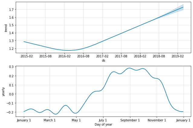
prophet1.plot_components(forecast_west)
plt.savefig('chart5.jpg')
prophet1.plot(forecast_west)
plt.savefig('chart6.jpg')

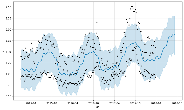
future_west_week = prophet1.make_future_dataframe(periods=24,freq='W')
forecast_west_week = prophet1.predict(future_west_week)
prophet1.plot(forecast_west_week)
plt.savefig('chart3.jpg')
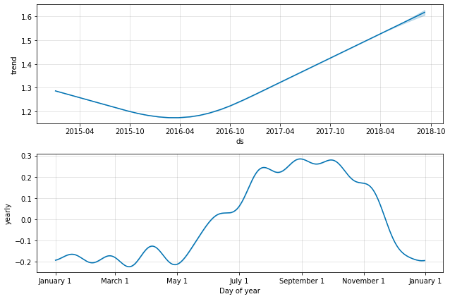
prophet1.plot_components(forecast_west_week)
plt.savefig('chart4.jpg')
댓글남기기