ANN을 이용한 가격 예측 -colab

2021-12-02 6 분 소요

자동차 구매 가격 예측

PROBLEM STATEMENT

다음과 같은 컬럼을 가지고 있는 데이터셋을 읽어서, 어떠한 고객이 있을때, 그 고객이 얼마정도의 차를 구매할 수 있을지를 예측하여, 그 사람에게 맞는 자동차를 보여주려 한다.

Customer Name
Customer e-mail
Country
Gender
Age
Annual Salary
Credit Card Debt
Net Worth (순자산)

예측하고자 하는 값 :

Car Purchase Amount

STEP #0: 라이브러리 임포트 및 코랩 환경 설정

구글 드라이브 파일 읽기 참고

import pandas as pd
import numpy as np
import matplotlib.pyplot as plt
import seaborn as sns

csv 파일을 읽기 위해, 구글 드라이브 마운트 하시오

from google.colab import drive
drive.mount('/content/drive')

Mounted at /content/drive

working directory 를, 현재의 파일이 속한 폴더로 셋팅하시오.

import os
os.chdir('/content/drive/MyDrive/python/day17')

STEP #1: IMPORT DATASET

Car_Purchasing_Data.csv 파일을 사용한다. 코랩의 경우 구글드라이브의 전체경로를 복사하여 파일 읽는다.

인코딩은 다음처럼 한다. encoding=’ISO-8859-1’

car_df = pd.read_csv('Car_Purchasing_Data.csv', encoding='ISO-8859-1')

컬럼을 확인하고

기본 통계 데이터를 확인해 보자

car_df

	Customer Name	Customer e-mail	Country	Gender	Age	Annual Salary	Credit Card Debt	Net Worth	Car Purchase Amount
0	Martina Avila	cubilia.Curae.Phasellus@quisaccumsanconvallis.edu	Bulgaria	0	41.851720	62812.09301	11609.380910	238961.2505	35321.45877
1	Harlan Barnes	eu.dolor@diam.co.uk	Belize	0	40.870623	66646.89292	9572.957136	530973.9078	45115.52566
2	Naomi Rodriquez	vulputate.mauris.sagittis@ametconsectetueradip...	Algeria	1	43.152897	53798.55112	11160.355060	638467.1773	42925.70921
3	Jade Cunningham	malesuada@dignissim.com	Cook Islands	1	58.271369	79370.03798	14426.164850	548599.0524	67422.36313
4	Cedric Leach	felis.ullamcorper.viverra@egetmollislectus.net	Brazil	1	57.313749	59729.15130	5358.712177	560304.0671	55915.46248
...	...	...	...	...	...	...	...	...	...
495	Walter	ligula@Cumsociis.ca	Nepal	0	41.462515	71942.40291	6995.902524	541670.1016	48901.44342
496	Vanna	Cum.sociis.natoque@Sedmolestie.edu	Zimbabwe	1	37.642000	56039.49793	12301.456790	360419.0988	31491.41457
497	Pearl	penatibus.et@massanonante.com	Philippines	1	53.943497	68888.77805	10611.606860	764531.3203	64147.28888
498	Nell	Quisque.varius@arcuVivamussit.net	Botswana	1	59.160509	49811.99062	14013.034510	337826.6382	45442.15353
499	Marla	Camaron.marla@hotmail.com	marlal	1	46.731152	61370.67766	9391.341628	462946.4924	45107.22566

500 rows × 9 columns

car_df.isna().sum()

Customer Name          0
Customer e-mail        0
Country                0
Gender                 0
Age                    0
Annual Salary          0
Credit Card Debt       0
Net Worth              0
Car Purchase Amount    0
dtype: int64

연봉이 가장 높은 사람은 누구인가

car_df[car_df['Annual Salary'] ==car_df['Annual Salary'].max()]

	Customer Name	Customer e-mail	Country	Gender	Age	Annual Salary	Credit Card Debt	Net Worth	Car Purchase Amount
28	Gemma Hendrix	lobortis@non.co.uk	Denmark	1	46.124036	100000.0	17452.92179	188032.0778	58350.31809

나이가 가장 어린 고객은, 연봉이 얼마인가

car_df[car_df['Age'] == car_df['Age'].min()]

	Customer Name	Customer e-mail	Country	Gender	Age	Annual Salary	Credit Card Debt	Net Worth	Car Purchase Amount
444	Camden	Aliquam.adipiscing.lobortis@loremut.net	Congo (Brazzaville)	1	20.0	70467.29492	100.0	494606.6334	28645.39425

STEP #2: VISUALIZE DATASET

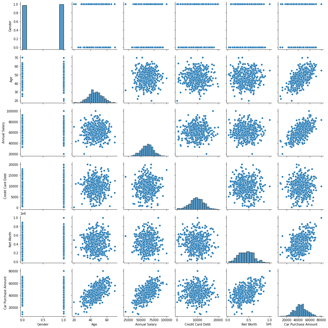
상관관계를 분석하기 위해, pairplot 을 그려보자.

sns.pairplot(car_df)

<seaborn.axisgrid.PairGrid at 0x7f0265add490>

png

car_df.corr()

	Gender	Age	Annual Salary	Credit Card Debt	Net Worth	Car Purchase Amount
Gender	1.000000	-0.064481	-0.036499	0.024193	-0.008395	-0.066408
Age	-0.064481	1.000000	0.000130	0.034721	0.020356	0.632865
Annual Salary	-0.036499	0.000130	1.000000	0.049599	0.014767	0.617862
Credit Card Debt	0.024193	0.034721	0.049599	1.000000	-0.049378	0.028882
Net Worth	-0.008395	0.020356	0.014767	-0.049378	1.000000	0.488580
Car Purchase Amount	-0.066408	0.632865	0.617862	0.028882	0.488580	1.000000

STEP #3: CREATE TESTING AND TRAINING DATASET/DATA CLEANING

NaN 값이 있으면, 이를 해결하시오.

car_df.isna().sum()

Customer Name          0
Customer e-mail        0
Country                0
Gender                 0
Age                    0
Annual Salary          0
Credit Card Debt       0
Net Worth              0
Car Purchase Amount    0
dtype: int64

학습을 위해 ‘Customer Name’, ‘Customer e-mail’, ‘Country’, ‘Car Purchase Amount’ 컬럼을 제외한 컬럼만, X로 만드시오.

car_df.head()

	Customer Name	Customer e-mail	Country	Gender	Age	Annual Salary	Credit Card Debt	Net Worth	Car Purchase Amount
0	Martina Avila	cubilia.Curae.Phasellus@quisaccumsanconvallis.edu	Bulgaria	0	41.851720	62812.09301	11609.380910	238961.2505	35321.45877
1	Harlan Barnes	eu.dolor@diam.co.uk	Belize	0	40.870623	66646.89292	9572.957136	530973.9078	45115.52566
2	Naomi Rodriquez	vulputate.mauris.sagittis@ametconsectetueradip...	Algeria	1	43.152897	53798.55112	11160.355060	638467.1773	42925.70921
3	Jade Cunningham	malesuada@dignissim.com	Cook Islands	1	58.271369	79370.03798	14426.164850	548599.0524	67422.36313
4	Cedric Leach	felis.ullamcorper.viverra@egetmollislectus.net	Brazil	1	57.313749	59729.15130	5358.712177	560304.0671	55915.46248

X = car_df.iloc[:,3:-1]

	Gender	Age	Annual Salary	Credit Card Debt	Net Worth
0	0	41.851720	62812.09301	11609.380910	238961.2505
1	0	40.870623	66646.89292	9572.957136	530973.9078
2	1	43.152897	53798.55112	11160.355060	638467.1773
3	1	58.271369	79370.03798	14426.164850	548599.0524
4	1	57.313749	59729.15130	5358.712177	560304.0671
...	...	...	...	...	...
495	0	41.462515	71942.40291	6995.902524	541670.1016
496	1	37.642000	56039.49793	12301.456790	360419.0988
497	1	53.943497	68888.77805	10611.606860	764531.3203
498	1	59.160509	49811.99062	14013.034510	337826.6382
499	1	46.731152	61370.67766	9391.341628	462946.4924

500 rows × 5 columns

y 값은 ‘Car Purchase Amount’ 컬럼으로 셋팅하시오.

y = car_df['Car Purchase Amount']

피처 스케일링 하겠습니다. 정규화(normalization)를 사용합니다. MinMaxScaler 를 이용하시오.

from sklearn.preprocessing import MinMaxScaler

scaler_X = MinMaxScaler()

X = scaler_X.fit_transform(X)

array([[0.        , 0.4370344 , 0.53515116, 0.57836085, 0.22342985],
       [0.        , 0.41741247, 0.58308616, 0.476028  , 0.52140195],
       [1.        , 0.46305795, 0.42248189, 0.55579674, 0.63108896],
       ...,
       [1.        , 0.67886994, 0.61110973, 0.52822145, 0.75972584],
       [1.        , 0.78321017, 0.37264988, 0.69914746, 0.3243129 ],
       [1.        , 0.53462305, 0.51713347, 0.46690159, 0.45198622]])

학습을 위해서, y 의 shape 을 변경하시오.

y = y.reshape(500,1)

y 도 피처 스케일링 하겠습니다. X 처럼 y도 노멀라이징 하시오.

scaler_y = MinMaxScaler()

y = scaler_y.fit_transform(y)

STEP#4: TRAINING THE MODEL

트레이닝셋과 테스트셋으로 분리하시오. (테스트 사이즈는 25%로 하며, 동일 결과를 위해 랜덤스테이트는 50 으로 셋팅하시오.)

from sklearn.model_selection import train_test_split

X_train,X_test,y_train,y_test=train_test_split(X,y,test_size=0.25,random_state=50)

아래 라이브러리를 임포트 하시오

import tensorflow.keras
from keras.models import Sequential
from keras.layers import Dense
from sklearn.preprocessing import MinMaxScaler

딥러닝을 이용한 모델링을 하시오.

model = Sequential()

model.add( Dense(units=6,activation='relu',input_dim=5) )

model.add( Dense(units=10,activation='relu') )

model.add( Dense(units=6,activation='relu') )

# 리그레션 문제의 액티베이션 펑션은 linear 사용
model.add(Dense(units=1,activation='linear'))

model.summary()

Model: "sequential_5"
_________________________________________________________________
 Layer (type)                Output Shape              Param #   
=================================================================
 dense_18 (Dense)            (None, 6)                 36        
                                                                 
 dense_19 (Dense)            (None, 10)                70        
                                                                 
 dense_20 (Dense)            (None, 6)                 66        
                                                                 
 dense_21 (Dense)            (None, 1)                 7         
                                                                 
=================================================================
Total params: 179
Trainable params: 179
Non-trainable params: 0
_________________________________________________________________

옵티마이저는 ‘adam’ 으로 하고, 로스펑션은 ‘mean_squared_error’ 로 셋팅하여 컴파일 하시오

model.compile(optimizer='adam',loss='mean_squared_error')

학습을 진행하시오.

epoch_history = model.fit(X_train,y_train, batch_size=20,epochs=29)

Epoch 1/29
19/19 [==============================] - 0s 2ms/step - loss: 0.0347
Epoch 2/29
19/19 [==============================] - 0s 2ms/step - loss: 0.0256
Epoch 3/29
19/19 [==============================] - 0s 2ms/step - loss: 0.0193
Epoch 4/29
19/19 [==============================] - 0s 2ms/step - loss: 0.0147
Epoch 5/29
19/19 [==============================] - 0s 2ms/step - loss: 0.0113
Epoch 6/29
19/19 [==============================] - 0s 2ms/step - loss: 0.0093
Epoch 7/29
19/19 [==============================] - 0s 2ms/step - loss: 0.0083
Epoch 8/29
19/19 [==============================] - 0s 2ms/step - loss: 0.0079
Epoch 9/29
19/19 [==============================] - 0s 2ms/step - loss: 0.0075
Epoch 10/29
19/19 [==============================] - 0s 2ms/step - loss: 0.0071
Epoch 11/29
19/19 [==============================] - 0s 2ms/step - loss: 0.0066
Epoch 12/29
19/19 [==============================] - 0s 2ms/step - loss: 0.0063
Epoch 13/29
19/19 [==============================] - 0s 2ms/step - loss: 0.0058
Epoch 14/29
19/19 [==============================] - 0s 2ms/step - loss: 0.0054
Epoch 15/29
19/19 [==============================] - 0s 2ms/step - loss: 0.0052
Epoch 16/29
19/19 [==============================] - 0s 2ms/step - loss: 0.0047
Epoch 17/29
19/19 [==============================] - 0s 2ms/step - loss: 0.0044
Epoch 18/29
19/19 [==============================] - 0s 2ms/step - loss: 0.0039
Epoch 19/29
19/19 [==============================] - 0s 2ms/step - loss: 0.0036
Epoch 20/29
19/19 [==============================] - 0s 2ms/step - loss: 0.0032
Epoch 21/29
19/19 [==============================] - 0s 2ms/step - loss: 0.0028
Epoch 22/29
19/19 [==============================] - 0s 2ms/step - loss: 0.0026
Epoch 23/29
19/19 [==============================] - 0s 2ms/step - loss: 0.0023
Epoch 24/29
19/19 [==============================] - 0s 2ms/step - loss: 0.0020
Epoch 25/29
19/19 [==============================] - 0s 2ms/step - loss: 0.0017
Epoch 26/29
19/19 [==============================] - 0s 2ms/step - loss: 0.0014
Epoch 27/29
19/19 [==============================] - 0s 2ms/step - loss: 0.0013
Epoch 28/29
19/19 [==============================] - 0s 2ms/step - loss: 0.0010
Epoch 29/29
19/19 [==============================] - 0s 2ms/step - loss: 8.6643e-04

STEP#5: EVALUATING THE MODEL

y_pred = model.predict(X_test)

# MSE : 오차를 구하고 제곱한 후 평균을 구한다
# Mean Squared Error
((y_test - y_pred)**2).mean()

0.0011123861375233498

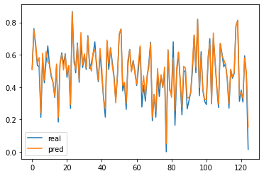
실제값과 예측값을 plot 으로 나타내시오.

plt.plot(y_test)
plt.plot(y_pred)
plt.legend(['real','pred'])
plt.show()

png

새로운 고객 데이터가 있습니다. 이 사람은 차량을 얼마정도 구매 가능한지 예측하시오.

여자이고, 나이는 38, 연봉은 90000, 카드빚은 2000, 순자산은 500000 일때, 어느정도의 차량을 구매할 수 있을지 예측하시오.

new_data = np.array([1,38,90000,2000,50000])

new_data = new_data.reshape(1,5)

new_data = scaler_X.transform(new_data)

y_pred = model.predict(new_data)

scaler_y.inverse_transform(y_pred)

array([[3.7154422e+09]], dtype=float32)

Twitter Facebook LinkedIn

ANN을 이용한 가격 예측 -colab

자동차 구매 가격 예측

PROBLEM STATEMENT

STEP #0: 라이브러리 임포트 및 코랩 환경 설정

STEP #1: IMPORT DATASET

STEP #2: VISUALIZE DATASET

STEP #3: CREATE TESTING AND TRAINING DATASET/DATA CLEANING

STEP#4: TRAINING THE MODEL

STEP#5: EVALUATING THE MODEL

공유하기

댓글남기기

참고

개발환경 설정 - Jupyter notebook

개발환경 설정 - Anaconda

Naive_Bayes를 이용한 리뷰 분류 -colab

Prophet을 이용한 가격예측 -colab