PYTHON PROGRAMMING FUNDAMENTALS
Pandas 의 장점
- Allows the use of labels for rows and columns
- 기본적인 통계데이터 제공
- NaN values 를 알아서 처리함.
- 숫자 문자열을 알아서 로드함.
- 데이터셋들을 merge 할 수 있음.
- It integrates with NumPy and Matplotlib
Pandas Series 데이터 생성하기
index = ['eggs', 'apples', 'milk', 'bread']
data = [30, 6, 'Yes', 'No']
# 용어 필수 암기 : 판다스의 1차원 데이터를 Series(시리즈) 라고 부른다.
0     30
1      6
2    Yes
3     No
dtype: object
# 시리즈의 왼쪽을 인덱스라고 부른다.
# 전에 리스트할때 배웠던 인덱스는, 컴퓨터가 자동으로 매기는 인덱스.
# 판다스에서 인덱스는! 사람용 인덱스!
# 시리즈의 오른쪽을 values라고 부른다.
groceries = pd.Series(data = data, index= index)
eggs       30
apples      6
milk      Yes
bread      No
dtype: object
Index(['eggs', 'apples', 'milk', 'bread'], dtype='object')
array([30, 6, 'Yes', 'No'], dtype=object)
Accessing and Deleting Elements in Pandas Series - 레이블과 인덱스
pandas.core.series.Series
eggs       30
apples      6
milk      Yes
bread      No
dtype: object
groceries[['eggs','bread']]
eggs     30
bread    No
dtype: object
eggs       30
apples      6
milk      Yes
dtype: object
eggs       30
apples      6
milk      Yes
dtype: object
Arithmetic Operations on Pandas Series
index = ['apples', 'oranges', 'bananas']
data = [10, 6, 3,]
fruits = pd.Series(data = data , index = index)
apples     10
oranges     6
bananas     3
dtype: int64
apples     15
oranges    11
bananas     8
dtype: int64
fruits['oranges'] = fruits['oranges'] - 2
apples     15
oranges     9
bananas     8
dtype: int64
# apple과 banana가 2개씩 더 늘었습니다. 이를 반영해주세요.
fruits[['apples','bananas']] = fruits[['apples','bananas']] + 2
apples     17
oranges     9
bananas    10
dtype: int64
실습
import pandas as pd
다음과 같은 레이블과 값을 가지는 Pandas Series 를 만드세요. 변수는 dist_planets 로 만드세요.
distance_from_sun = [149.6, 1433.5, 227.9, 108.2, 778.6]
planets = [‘Earth’,’Saturn’, ‘Mars’,’Venus’, ‘Jupiter’]
dist_planets =
-
거리를 빛의 상수 c( 18 ) 로 나눠서, 가는 시간이 얼마나 걸리는 지 계산하여 저장하세요.
time_light =
-
Boolean indexing을 이용해서 가는 시간이 40분보다 작은것들만 셀렉트 하세요.
close_planets =
distance_from_sun = [149.6, 1433.5, 227.9, 108.2, 778.6]
planets = ['Earth','Saturn', 'Mars','Venus', 'Jupiter']
dist_planets = pd.Series(data = distance_from_sun,index = planets)
Earth       149.6
Saturn     1433.5
Mars        227.9
Venus       108.2
Jupiter     778.6
dtype: float64
time_light = dist_planets / 18
Earth       8.311111
Saturn     79.638889
Mars       12.661111
Venus       6.011111
Jupiter    43.255556
dtype: float64
close_planets = time_light[time_light.values < 40]
Earth     8.311111
Mars     12.661111
Venus     6.011111
dtype: float64
Pandas Dataframe
레이블로 생성하기
import pandas as pd

# We create a dictionary of Pandas Series
items = {'Bob' : pd.Series(data = [245, 25, 55], index = ['bike', 'pants', 'watch']),
         'Alice' : pd.Series(data = [40, 110, 500, 45], index = ['book', 'glasses', 'bike', 'pants'])}
df = pd.DataFrame(data= items)
# 용어 : 데이터 프레임은 인덱스와 컬럼과 벨류로 되어있다.
# DataFrame, index , columns, values
NaN 은 해당 항목에 값이 없음을 뜻합니다. (Not a Number)
|
Bob |
Alice |
| bike |
245.0 |
500.0 |
| book |
NaN |
40.0 |
| glasses |
NaN |
110.0 |
| pants |
25.0 |
45.0 |
| watch |
55.0 |
NaN |
Index(['bike', 'book', 'glasses', 'pants', 'watch'], dtype='object')
array([[245., 500.],
       [ nan,  40.],
       [ nan, 110.],
       [ 25.,  45.],
       [ 55.,  nan]])
인덱스 및 컬럼 생성하기
items = {'Bob' : pd.Series(data = [245, 25, 55], index = ['bike', 'pants', 'watch']),
         'Alice' : pd.Series(data = [40, 110, 500, 45], index = ['book', 'glasses', 'bike', 'pants'])}
# 실제로 데이터 분석은 파일을 읽어서 판다스 테이터프레임으로 만들고 분석을 한다.
# 가장 기본적인 파일 형식은 csv 파일이다.
# csv파일을 읽어서 데이터프레임으로 변환하여 사용한다.
df = pd.read_csv('test.csv')
|
name |
age |
salary |
| 0 |
홍길동 |
25 |
3000 |
| 1 |
김나나 |
33 |
5000 |
| 2 |
진달래 |
40 |
8000 |
pd.read_csv('my_file.csv',index_col= 0 )
|
name |
age |
salary |
| 0 |
홍길동 |
25 |
3000 |
| 1 |
김나나 |
33 |
5000 |
| 2 |
진달래 |
40 |
8000 |
pd.read_csv('my_file.csv')
|
Unnamed: 0 |
name |
age |
salary |
| 0 |
0 |
홍길동 |
25 |
3000 |
| 1 |
1 |
김나나 |
33 |
5000 |
| 2 |
2 |
진달래 |
40 |
8000 |
pd.read_csv('my_file.csv',index_col= 'Unnamed: 0' )
|
name |
age |
salary |
| 0 |
홍길동 |
25 |
3000 |
| 1 |
김나나 |
33 |
5000 |
| 2 |
진달래 |
40 |
8000 |
Accessing Elements in Pandas DataFrames
# We create a list of Python dictionaries
items2 = [{'bikes': 20, 'pants': 30, 'watches': 35},
          {'watches': 10, 'glasses': 50, 'bikes': 15, 'pants':5}]
df = pd.DataFrame(data = items2, index = ["store 1","store 2"])
|
bikes |
pants |
watches |
glasses |
| store 1 |
20 |
30 |
35 |
NaN |
| store 2 |
15 |
5 |
10 |
50.0 |
### 중요!! 데이터 프레임에서, 데이터를 억세스하는 방법
#### 3가지!

# 데이터 억세스 기호는 대괄호!

# 1. 컬럼의 값을 가져오는 방법
store 1    30
store 2     5
Name: pants, dtype: int64
store 1    30
store 2     5
Name: pants, dtype: int64
|
pants |
glasses |
| store 1 |
30 |
NaN |
| store 2 |
5 |
50.0 |
## 2. 행과 열의 정보로, 데이터를 가져오는 방법

## 2-1. 사람용인 인덱스와 컬럼명으로 데이터 억세스 하는 방법
##      => .loc[ , ]
|
bikes |
pants |
watches |
glasses |
| store 1 |
20 |
30 |
35 |
NaN |
| store 2 |
15 |
5 |
10 |
50.0 |
bikes      20.0
pants      30.0
watches    35.0
glasses     NaN
Name: store 1, dtype: float64
df.loc['store 1','pants']
# 스토어1의 바이크와 와치 데이터를 가져와라.
df.loc['store 1',['bikes','watches']]
bikes      20.0
watches    35.0
Name: store 1, dtype: float64
#스토어2에서 팬츠부터 글래시스 까지 데이터를 가져오시오
df.loc['store 2','pants':'glasses']
pants       5.0
watches    10.0
glasses    50.0
Name: store 2, dtype: float64
## 3. 행과 열의 정보로, 데이터를 가져오는 방법

## 3-1. 컴퓨터가 자동으로 매기는 인덱스로 행과 열을 이용하여 데이터 억세스 하는 방법
##      => .iloc[ , ]
|
bikes |
pants |
watches |
glasses |
| store 1 |
20 |
30 |
35 |
NaN |
| store 2 |
15 |
5 |
10 |
50.0 |
# 스토어 1의 바이크와 와치의 데이터를 가져오시오.
bikes      20.0
watches    35.0
Name: store 1, dtype: float64
# 스토어 1 데이터중, 팬츠부터 글래시스까지 가져오시오
pants      30.0
watches    35.0
glasses     NaN
Name: store 1, dtype: float64
|
bikes |
pants |
watches |
glasses |
| store 1 |
20 |
30 |
35 |
NaN |
| store 2 |
15 |
5 |
10 |
50.0 |
|
bikes |
pants |
watches |
glasses |
| store 1 |
20 |
30 |
35 |
NaN |
| store 2 |
15 |
5 |
20 |
50.0 |
|
bikes |
pants |
watches |
glasses |
| store 1 |
20 |
30 |
35 |
NaN |
| store 2 |
15 |
5 |
10 |
50.0 |
df.loc['store 1','watches'] = 25
|
bikes |
pants |
watches |
glasses |
| store 1 |
20 |
30 |
25 |
NaN |
| store 2 |
15 |
5 |
10 |
50.0 |
# shirts 컬럼을 만들자. store 1 에는 15개, stroe 2에는 2개를 넣자.
|
bikes |
pants |
watches |
glasses |
shirts |
| store 1 |
20 |
30 |
25 |
NaN |
15 |
| store 2 |
15 |
5 |
10 |
50.0 |
2 |
# suits 라는 컬럼을 만들건데 , pants이 수와 shirets의 수를 더해서 만드세요.
df['suits'] = df['pants'] + df['shirts']
|
bikes |
pants |
watches |
glasses |
shirts |
suits |
| store 1 |
20 |
30 |
25 |
NaN |
15 |
45 |
| store 2 |
15 |
5 |
10 |
50.0 |
2 |
7 |
new_item = [{'bikes' : 20,'pants': 30,'watches' : 35, 'glasses' : 4}]
new_store = pd.DataFrame(data = new_item, index=['store 3'])
|
bikes |
pants |
watches |
glasses |
| store 3 |
20 |
30 |
35 |
4 |
df = df.append(new_store)
|
bikes |
pants |
watches |
glasses |
shirts |
suits |
| store 1 |
20 |
30 |
25 |
NaN |
15.0 |
45.0 |
| store 2 |
15 |
5 |
10 |
50.0 |
2.0 |
7.0 |
| store 3 |
20 |
30 |
35 |
4.0 |
NaN |
NaN |
# 행삭제, 열삭제
# 인덱스 삭제, 컬럼 삭제
|
bikes |
pants |
watches |
glasses |
shirts |
suits |
| store 1 |
20 |
30 |
25 |
NaN |
15.0 |
45.0 |
| store 2 |
15 |
5 |
10 |
50.0 |
2.0 |
7.0 |
| store 3 |
20 |
30 |
35 |
4.0 |
NaN |
NaN |
df.drop('store 2', axis = 0)
|
bikes |
pants |
watches |
glasses |
shirts |
suits |
| store 1 |
20 |
30 |
25 |
NaN |
15.0 |
45.0 |
| store 3 |
20 |
30 |
35 |
4.0 |
NaN |
NaN |
df.drop('glasses', axis = 1)
|
bikes |
pants |
watches |
shirts |
suits |
| store 1 |
20 |
30 |
25 |
15.0 |
45.0 |
| store 2 |
15 |
5 |
10 |
2.0 |
7.0 |
| store 3 |
20 |
30 |
35 |
NaN |
NaN |
df.drop(['bikes','glasses','suits'],axis = 1)
|
pants |
watches |
shirts |
| store 1 |
30 |
25 |
15.0 |
| store 2 |
5 |
10 |
2.0 |
| store 3 |
30 |
35 |
NaN |
df.rename(index = {'store 3' : 'last store'})
|
bikes |
pants |
watches |
glasses |
shirts |
suits |
| store 1 |
20 |
30 |
25 |
NaN |
15.0 |
45.0 |
| store 2 |
15 |
5 |
10 |
50.0 |
2.0 |
7.0 |
| last store |
20 |
30 |
35 |
4.0 |
NaN |
NaN |
df.rename(columns = {'bikes' : 'hat','suits':'shoes'})
|
hat |
pants |
watches |
glasses |
shirts |
shoes |
| store 1 |
20 |
30 |
25 |
NaN |
15.0 |
45.0 |
| store 2 |
15 |
5 |
10 |
50.0 |
2.0 |
7.0 |
| store 3 |
20 |
30 |
35 |
4.0 |
NaN |
NaN |
# 새로운 컬럼 name 컬럼을 만드세요. A,B,C 로 데이터 셋팅하세요.
df['name'] = ['A','B','C']
|
bikes |
pants |
watches |
glasses |
shirts |
suits |
name |
| store 1 |
20 |
30 |
25 |
NaN |
15.0 |
45.0 |
A |
| store 2 |
15 |
5 |
10 |
50.0 |
2.0 |
7.0 |
B |
| store 3 |
20 |
30 |
35 |
4.0 |
NaN |
NaN |
C |
df = df.set_index('name')
|
bikes |
pants |
watches |
glasses |
shirts |
suits |
| name |
|
|
|
|
|
|
| A |
20 |
30 |
25 |
NaN |
15.0 |
45.0 |
| B |
15 |
5 |
10 |
50.0 |
2.0 |
7.0 |
| C |
20 |
30 |
35 |
4.0 |
NaN |
NaN |
df[['glasses','bikes','suits','name','watches','shirts','pants']]
|
glasses |
bikes |
suits |
name |
watches |
shirts |
pants |
| 0 |
NaN |
20 |
45.0 |
A |
25 |
15.0 |
30 |
| 1 |
50.0 |
15 |
7.0 |
B |
10 |
2.0 |
5 |
| 2 |
4.0 |
20 |
NaN |
C |
35 |
NaN |
30 |
Dealing with NaN
# We create a list of Python dictionaries
items2 = [{'bikes': 20, 'pants': 30, 'watches': 35, 'shirts': 15, 'shoes':8, 'suits':45},
{'watches': 10, 'glasses': 50, 'bikes': 15, 'pants':5, 'shirts': 2, 'shoes':5, 'suits':7},
{'bikes': 20, 'pants': 30, 'watches': 35, 'glasses': 4, 'shoes':10}]
df = pd.DataFrame(data = items2, index = ['store 1','store 2','store 3'])
|
bikes |
pants |
watches |
shirts |
shoes |
suits |
glasses |
| store 1 |
20 |
30 |
35 |
15.0 |
8 |
45.0 |
NaN |
| store 2 |
15 |
5 |
10 |
2.0 |
5 |
7.0 |
50.0 |
| store 3 |
20 |
30 |
35 |
NaN |
10 |
NaN |
4.0 |
# 컬럼별로 Nan 확인하는 방법
df.isna().sum()
bikes      0
pants      0
watches    0
shirts     1
shoes      0
suits      1
glasses    1
dtype: int64
# 데이터프레임 전체로 비어있는 항목의 갯수를 알고싶을때?
|
bikes |
pants |
watches |
shirts |
shoes |
suits |
glasses |
| store 1 |
20 |
30 |
35 |
15.0 |
8 |
45.0 |
NaN |
| store 2 |
15 |
5 |
10 |
2.0 |
5 |
7.0 |
50.0 |
| store 3 |
20 |
30 |
35 |
NaN |
10 |
NaN |
4.0 |
|
bikes |
pants |
watches |
shirts |
shoes |
suits |
glasses |
| store 2 |
15 |
5 |
10 |
2.0 |
5 |
7.0 |
50.0 |
# 열 삭제
df.dropna(axis = 1)
|
bikes |
pants |
watches |
shoes |
| store 1 |
20 |
30 |
35 |
8 |
| store 2 |
15 |
5 |
10 |
5 |
| store 3 |
20 |
30 |
35 |
10 |
|
bikes |
pants |
watches |
shirts |
shoes |
suits |
glasses |
| store 1 |
20 |
30 |
35 |
15.0 |
8 |
45.0 |
NaN |
| store 2 |
15 |
5 |
10 |
2.0 |
5 |
7.0 |
50.0 |
| store 3 |
20 |
30 |
35 |
NaN |
10 |
NaN |
4.0 |
|
bikes |
pants |
watches |
shirts |
shoes |
suits |
glasses |
| store 1 |
20 |
30 |
35 |
15.0 |
8 |
45.0 |
없음 |
| store 2 |
15 |
5 |
10 |
2.0 |
5 |
7.0 |
50.0 |
| store 3 |
20 |
30 |
35 |
없음 |
10 |
없음 |
4.0 |
# 셔츠칼럼의 데이터가 없는 경우는 No Data로 채워라
df['shirts'].fillna("No Data")
store 1       15.0
store 2        2.0
store 3    No Data
Name: shirts, dtype: object
|
bikes |
pants |
watches |
shirts |
shoes |
suits |
glasses |
| store 1 |
20 |
30 |
35 |
15.0 |
8 |
45.0 |
NaN |
| store 2 |
15 |
5 |
10 |
2.0 |
5 |
7.0 |
50.0 |
| store 3 |
20 |
30 |
35 |
NaN |
10 |
NaN |
4.0 |
# 앞의 데이터나 뒤의 데이터로 Nan 대체하는 방법
# ffill => foward fill
df.fillna(method= 'ffill', axis = 1)
|
bikes |
pants |
watches |
shirts |
shoes |
suits |
glasses |
| store 1 |
20.0 |
30.0 |
35.0 |
15.0 |
8.0 |
45.0 |
45.0 |
| store 2 |
15.0 |
5.0 |
10.0 |
2.0 |
5.0 |
7.0 |
50.0 |
| store 3 |
20.0 |
30.0 |
35.0 |
35.0 |
10.0 |
10.0 |
4.0 |
# bfill => backward fill
df.fillna(method= 'bfill', axis = 1)
|
bikes |
pants |
watches |
shirts |
shoes |
suits |
glasses |
| store 1 |
20.0 |
30.0 |
35.0 |
15.0 |
8.0 |
45.0 |
NaN |
| store 2 |
15.0 |
5.0 |
10.0 |
2.0 |
5.0 |
7.0 |
50.0 |
| store 3 |
20.0 |
30.0 |
35.0 |
10.0 |
10.0 |
4.0 |
4.0 |
# 채우는 전략중, 각 컬럼별로 최대값으로 채우기
# 각 컬럼별로 최소값으로 채우기
# 각 컬럼별로 그 컬럼의 평균값으로 채우기
|
bikes |
pants |
watches |
shirts |
shoes |
suits |
glasses |
| store 1 |
20 |
30 |
35 |
15.0 |
8 |
45.0 |
50.0 |
| store 2 |
15 |
5 |
10 |
2.0 |
5 |
7.0 |
50.0 |
| store 3 |
20 |
30 |
35 |
15.0 |
10 |
45.0 |
4.0 |
|
bikes |
pants |
watches |
shirts |
shoes |
suits |
glasses |
| store 1 |
20 |
30 |
35 |
15.0 |
8 |
45.0 |
4.0 |
| store 2 |
15 |
5 |
10 |
2.0 |
5 |
7.0 |
50.0 |
| store 3 |
20 |
30 |
35 |
2.0 |
10 |
7.0 |
4.0 |
|
bikes |
pants |
watches |
shirts |
shoes |
suits |
glasses |
| store 1 |
20 |
30 |
35 |
15.0 |
8 |
45.0 |
27.0 |
| store 2 |
15 |
5 |
10 |
2.0 |
5 |
7.0 |
50.0 |
| store 3 |
20 |
30 |
35 |
8.5 |
10 |
26.0 |
4.0 |
|
bikes |
pants |
watches |
shirts |
shoes |
suits |
glasses |
| store 1 |
True |
True |
True |
True |
True |
True |
False |
| store 2 |
True |
True |
True |
True |
True |
True |
True |
| store 3 |
True |
True |
True |
False |
True |
False |
True |
실습
import pandas as pd
import numpy as np

# 각 유저별 별점을 주는것이므로, 1 decimal 로 셋팅.
pd.set_option('precision', 1)

# 책 제목과 작가, 그리고 유저별 별점 데이터가 있다.

books = pd.Series(data = ['Great Expectations', 'Of Mice and Men', 'Romeo and Juliet', 'The Time Machine', 'Alice in Wonderland' ])
authors = pd.Series(data = ['Charles Dickens', 'John Steinbeck', 'William Shakespeare', ' H. G. Wells', 'Lewis Carroll' ])

user_1 = pd.Series(data = [3.2, np.nan ,2.5])
user_2 = pd.Series(data = [5., 1.3, 4.0, 3.8])
user_3 = pd.Series(data = [2.0, 2.3, np.nan, 4])
user_4 = pd.Series(data = [4, 3.5, 4, 5, 4.2])

#  np.nan values 는 해당 유저가 해당 책에는 아직 별점 주지 않은것이다.
# labels: 'Author', 'Book Title', 'User 1', 'User 2', 'User 3', 'User 4'.
# 아래 그림처럼 나오도록 만든다.

# 1. 딕셔너리를 만들고, 2. 데이터프레임으로 만든 후, 3. nan을 평균값으로 채운다.
my_data = {"Book Title":books,"Author":authors,"User1":user_1,"User2":user_2,"User3":user_3,"User4":user_4}
df = pd.DataFrame(data = my_data)
User1    2.9
User2    3.5
User3    2.8
User4    4.1
dtype: float64
|
Book Title |
Author |
User1 |
User2 |
User3 |
User4 |
| 0 |
Great Expectations |
Charles Dickens |
3.2 |
5.0 |
2.0 |
4.0 |
| 1 |
Of Mice and Men |
John Steinbeck |
2.9 |
1.3 |
2.3 |
3.5 |
| 2 |
Romeo and Juliet |
William Shakespeare |
2.5 |
4.0 |
2.8 |
4.0 |
| 3 |
The Time Machine |
H. G. Wells |
2.9 |
3.8 |
4.0 |
5.0 |
| 4 |
Alice in Wonderland |
Lewis Carroll |
2.9 |
3.5 |
2.8 |
4.2 |
Loading Data into a Pandas DataFrame
# Csv(Comma Separted Values) 파일을 읽는 방법
df = pd.read_csv("GOOG.csv")
|
Date |
Open |
High |
Low |
Close |
Adj Close |
Volume |
| 0 |
2004-08-19 |
49.7 |
51.7 |
47.7 |
49.8 |
49.8 |
44994500 |
| 1 |
2004-08-20 |
50.2 |
54.2 |
49.9 |
53.8 |
53.8 |
23005800 |
| 2 |
2004-08-23 |
55.0 |
56.4 |
54.2 |
54.3 |
54.3 |
18393200 |
| 3 |
2004-08-24 |
55.3 |
55.4 |
51.5 |
52.1 |
52.1 |
15361800 |
| 4 |
2004-08-25 |
52.1 |
53.7 |
51.6 |
52.7 |
52.7 |
9257400 |
Date         0
Open         0
High         0
Low          0
Close        0
Adj Close    0
Volume       0
dtype: int64
|
Open |
High |
Low |
Close |
Adj Close |
Volume |
| count |
3313.0 |
3313.0 |
3313.0 |
3313.0 |
3313.0 |
3.3e+03 |
| mean |
380.2 |
383.5 |
376.5 |
380.1 |
380.1 |
8.0e+06 |
| std |
223.8 |
225.0 |
222.5 |
223.9 |
223.9 |
8.4e+06 |
| min |
49.3 |
50.5 |
47.7 |
49.7 |
49.7 |
7.9e+03 |
| 25% |
226.6 |
228.4 |
224.0 |
226.4 |
226.4 |
2.6e+06 |
| 50% |
293.3 |
295.4 |
289.9 |
293.0 |
293.0 |
5.3e+06 |
| 75% |
536.7 |
540.0 |
532.4 |
536.7 |
536.7 |
1.1e+07 |
| max |
992.0 |
997.2 |
989.0 |
989.7 |
989.7 |
8.3e+07 |
<class 'pandas.core.frame.DataFrame'>
RangeIndex: 3313 entries, 0 to 3312
Data columns (total 7 columns):
 #   Column     Non-Null Count  Dtype
---  ------     --------------  -----
 0   Date       3313 non-null   object
 1   Open       3313 non-null   float64
 2   High       3313 non-null   float64
 3   Low        3313 non-null   float64
 4   Close      3313 non-null   float64
 5   Adj Close  3313 non-null   float64
 6   Volume     3313 non-null   int64
dtypes: float64(5), int64(1), object(1)
memory usage: 181.3+ KB
count    3313.0
mean      383.5
std       225.0
min        50.5
25%       228.4
50%       295.4
75%       540.0
max       997.2
Name: High, dtype: float64
df[['Open','High']].describe()
|
Open |
High |
| count |
3313.0 |
3313.0 |
| mean |
380.2 |
383.5 |
| std |
223.8 |
225.0 |
| min |
49.3 |
50.5 |
| 25% |
226.6 |
228.4 |
| 50% |
293.3 |
295.4 |
| 75% |
536.7 |
540.0 |
| max |
992.0 |
997.2 |
df= pd.read_csv('fake_company.csv')
|
Year |
Name |
Department |
Age |
Salary |
| 0 |
1990 |
Alice |
HR |
25 |
50000 |
| 1 |
1990 |
Bob |
RD |
30 |
48000 |
| 2 |
1990 |
Charlie |
Admin |
45 |
55000 |
| 3 |
1991 |
Alice |
HR |
26 |
52000 |
| 4 |
1991 |
Bob |
RD |
31 |
50000 |
| 5 |
1991 |
Charlie |
Admin |
46 |
60000 |
| 6 |
1992 |
Alice |
HR |
27 |
60000 |
| 7 |
1992 |
Bob |
RD |
32 |
52000 |
| 8 |
1992 |
Charlie |
Admin |
47 |
62000 |
|
Year |
Name |
Department |
Age |
Salary |
| 0 |
1990 |
Alice |
HR |
25 |
50000 |
| 1 |
1990 |
Bob |
RD |
30 |
48000 |
| 2 |
1990 |
Charlie |
Admin |
45 |
55000 |
| 3 |
1991 |
Alice |
HR |
26 |
52000 |
| 4 |
1991 |
Bob |
RD |
31 |
50000 |
|
Year |
Name |
Department |
Age |
Salary |
| 4 |
1991 |
Bob |
RD |
31 |
50000 |
| 5 |
1991 |
Charlie |
Admin |
46 |
60000 |
| 6 |
1992 |
Alice |
HR |
27 |
60000 |
| 7 |
1992 |
Bob |
RD |
32 |
52000 |
| 8 |
1992 |
Charlie |
Admin |
47 |
62000 |
|
Year |
Age |
Salary |
| count |
9.0 |
9.0 |
9.0 |
| mean |
1991.0 |
34.3 |
54333.3 |
| std |
0.9 |
9.1 |
5147.8 |
| min |
1990.0 |
25.0 |
48000.0 |
| 25% |
1990.0 |
27.0 |
50000.0 |
| 50% |
1991.0 |
31.0 |
52000.0 |
| 75% |
1992.0 |
45.0 |
60000.0 |
| max |
1992.0 |
47.0 |
62000.0 |
<class 'pandas.core.frame.DataFrame'>
RangeIndex: 9 entries, 0 to 8
Data columns (total 5 columns):
 #   Column      Non-Null Count  Dtype
---  ------      --------------  -----
 0   Year        9 non-null      int64
 1   Name        9 non-null      object
 2   Department  9 non-null      object
 3   Age         9 non-null      int64
 4   Salary      9 non-null      int64
dtypes: int64(3), object(2)
memory usage: 488.0+ bytes
# 카테고리컬 데이터 (categorical data)
|
Year |
Name |
Department |
Age |
Salary |
| 0 |
1990 |
Alice |
HR |
25 |
50000 |
| 1 |
1990 |
Bob |
RD |
30 |
48000 |
| 2 |
1990 |
Charlie |
Admin |
45 |
55000 |
| 3 |
1991 |
Alice |
HR |
26 |
52000 |
| 4 |
1991 |
Bob |
RD |
31 |
50000 |
| 5 |
1991 |
Charlie |
Admin |
46 |
60000 |
| 6 |
1992 |
Alice |
HR |
27 |
60000 |
| 7 |
1992 |
Bob |
RD |
32 |
52000 |
| 8 |
1992 |
Charlie |
Admin |
47 |
62000 |
# 카테고리컬 데이터를 분선할 수 있는 함수들 설명
array([1990, 1991, 1992], dtype=int64)
array(['Alice', 'Bob', 'Charlie'], dtype=object)
df['Department'].nunique()
df['Department'].unique()
array(['HR', 'RD', 'Admin'], dtype=object)
# 문자열 컬럼은, 각각 해당 컬럼에 describe 해준다.
count       9
unique      3
top       Bob
freq        3
Name: Name, dtype: object
df['Department'].describe()
count         9
unique        3
top       Admin
freq          3
Name: Department, dtype: object
# 카테고리컬 데이터의 각 데이터별로 묶어서 처리하는 함수
df.groupby('Year')['Salary'].sum()
Year
1990    153000
1991    162000
1992    174000
Name: Salary, dtype: int64
# 각 직원별로 연봉을 평균 얼마씩 받았는지 구하시오.
df.groupby('Name')['Salary'].mean()
Name
Alice      54000
Bob        50000
Charlie    59000
Name: Salary, dtype: int64
# 년도별, 부서별로 연봉은 총 얼마씩 지급하였는지 구하세요.
df.groupby(['Year','Department'])['Salary'].sum()
Year  Department
1990  Admin         55000
      HR            50000
      RD            48000
1991  Admin         60000
      HR            52000
      RD            50000
1992  Admin         62000
      HR            60000
      RD            52000
Name: Salary, dtype: int64
# 년도별 연봉 총합과 평균을 구하세요.
# agg => 집계
df.groupby('Year')['Salary'].agg(([np.sum,np.mean,np.std]))
|
sum |
mean |
std |
| Year |
|
|
|
| 1990 |
153000 |
51000 |
3605.6 |
| 1991 |
162000 |
54000 |
5291.5 |
| 1992 |
174000 |
58000 |
5291.5 |
# 카테고리컬 데이터의, 데이터별로 갯수를 세어주는 함수
# Name 컬럼의 데이터가 각각 몇개씩 있는지 확인
df['Name'].value_counts()
Bob        3
Alice      3
Charlie    3
Name: Name, dtype: int64
df['Department'].value_counts()
Admin    3
RD       3
HR       3
Name: Department, dtype: int64
GETTING HTML DATA
# 웹 페이지에서 표로 되어있는 부분을 데이터 프레임으로 가져오는 방법
df = pd.read_html('https://www.livingin-canada.com/house-prices-canada.html')
|
City |
Average House Price |
12 Month Change |
| 0 |
Vancouver, BC |
$1,036,000 |
+ 2.63 % |
| 1 |
Toronto, Ont |
$870,000 |
+10.2 % |
| 2 |
Ottawa, Ont |
$479,000 |
+ 15.4 % |
| 3 |
Calgary, Alb |
$410,000 |
– 1.5 % |
| 4 |
Montreal, Que |
$435,000 |
+ 9.3 % |
| 5 |
Halifax, NS |
$331,000 |
+ 3.6 % |
| 6 |
Regina, Sask |
$254,000 |
– 3.9 % |
| 7 |
Fredericton, NB |
$198,000 |
– 4.3 % |
|
Province |
Average House Price |
12 Month Change |
| 0 |
British Columbia |
$736,000 |
+ 7.6 % |
| 1 |
Ontario |
$594,000 |
– 3.2 % |
| 2 |
Alberta |
$353,000 |
– 7.5 % |
| 3 |
Quebec |
$340,000 |
+ 7.6 % |
| 4 |
Manitoba |
$295,000 |
– 1.4 % |
| 5 |
Saskatchewan |
$271,000 |
– 3.8 % |
| 6 |
Nova Scotia |
$266,000 |
+ 3.5 % |
| 7 |
Prince Edward Island |
$243,000 |
+ 3.0 % |
| 8 |
Newfoundland / Labrador |
$236,000 |
– 1.6 % |
| 9 |
New Brunswick |
$183,000 |
– 2.2 % |
| 10 |
Canadian Average |
$488,000 |
– 1.3 % |
PANDAS OPERATIONS
df = pd.DataFrame({'Employee ID':[111, 222, 333, 444],
                   'Employee Name':['Chanel', 'Steve', 'Mitch', 'Bird'],
                   'Salary [$/h]':[35, 29, 38, 20],
                   'Years of Experience':[3, 4 ,9, 1]})
df
|
Employee ID |
Employee Name |
Salary [$/h] |
Years of Experience |
| 0 |
111 |
Chanel |
35 |
3 |
| 1 |
222 |
Steve |
29 |
4 |
| 2 |
333 |
Mitch |
38 |
9 |
| 3 |
444 |
Bird |
20 |
1 |
# 경력이 3년 이상인 사람의 데이터{행을 가져와라]를 가져와라.
df.loc[df['Years of Experience'] >= 3 , ]
|
Employee ID |
Employee Name |
Salary [$/h] |
Years of Experience |
| 0 |
111 |
Chanel |
35 |
3 |
| 1 |
222 |
Steve |
29 |
4 |
| 2 |
333 |
Mitch |
38 |
9 |
#경력이 3년 이상인 사람의 이름과 시급을 가져오시오.
df.loc[df['Years of Experience'] >= 3 ,['Employee Name','Salary [$/h]']]
|
Employee Name |
Salary [$/h] |
| 0 |
Chanel |
35 |
| 1 |
Steve |
29 |
| 2 |
Mitch |
38 |
# 경력이 3년 이상이고, 시급이 30달러 이상인 사람의 데이터는?
df.loc[(df['Years of Experience'] >= 3) & (df['Salary [$/h]'] >= 30), ]
|
Employee ID |
Employee Name |
Salary [$/h] |
Years of Experience |
| 0 |
111 |
Chanel |
35 |
3 |
| 2 |
333 |
Mitch |
38 |
9 |
# 경력이 3년 이하이거나 8년 이상인 사람의 이름을 가져오시오.
years = (df['Years of Experience'] <= 3) | (df['Years of Experience'] >= 8)
df.loc[years, "Employee Name"]
0    Chanel
2     Mitch
3      Bird
Name: Employee Name, dtype: object
df.loc[(df['Salary [$/h]']) == (df['Salary [$/h]'].max()),"Employee Name"]
2    Mitch
Name: Employee Name, dtype: object
APPLYING FUNCTIONS
|
Employee ID |
Employee Name |
Salary [$/h] |
Years of Experience |
| 0 |
111 |
Chanel |
35 |
3 |
| 1 |
222 |
Steve |
29 |
4 |
| 2 |
333 |
Mitch |
38 |
9 |
| 3 |
444 |
Bird |
20 |
1 |
# 직원 이름이 몇글자인지 , 글자수를 세어서, 새로운 컬럼 length
# 컬럼에 저장하세요
df['length'] = df['Employee Name'].apply( len )
|
Employee ID |
Employee Name |
Salary [$/h] |
Years of Experience |
length |
| 0 |
111 |
Chanel |
35 |
3 |
6 |
| 1 |
222 |
Steve |
29 |
4 |
5 |
| 2 |
333 |
Mitch |
38 |
9 |
5 |
| 3 |
444 |
Bird |
20 |
1 |
4 |
# 시급이 30보다 이상이면 'A'라고 하고
# 시급이 30보다 미만이면 'B'라고 하여, 그룹을 구분할 것.
# 이 정보를 새로운 컬럼 '그룹' 이라고 하여 저장
def group(salary):
    if salary >= 30:
        return "A"
    else:
        return "B"
df['Gruoup']= df["Salary [$/h]"].apply( group )
|
Employee ID |
Employee Name |
Salary [$/h] |
Years of Experience |
length |
Gruoup |
| 0 |
111 |
Chanel |
35 |
3 |
6 |
A |
| 1 |
222 |
Steve |
29 |
4 |
5 |
B |
| 2 |
333 |
Mitch |
38 |
9 |
5 |
A |
| 3 |
444 |
Bird |
20 |
1 |
4 |
B |
SORTING AND ORDERING
df = pd.DataFrame({'Employee ID':[111, 222, 333, 444],
                   'Employee Name':['Chanel', 'Steve', 'Mitch', 'Bird'],
                   'Salary [$/h]':[35, 29, 38, 20],
                   'Years of Experience':[3, 4 ,9, 1]})
df
|
Employee ID |
Employee Name |
Salary [$/h] |
Years of Experience |
| 0 |
111 |
Chanel |
35 |
3 |
| 1 |
222 |
Steve |
29 |
4 |
| 2 |
333 |
Mitch |
38 |
9 |
| 3 |
444 |
Bird |
20 |
1 |
df.sort_values('Years of Experience')
|
Employee ID |
Employee Name |
Salary [$/h] |
Years of Experience |
| 3 |
444 |
Bird |
20 |
1 |
| 0 |
111 |
Chanel |
35 |
3 |
| 1 |
222 |
Steve |
29 |
4 |
| 2 |
333 |
Mitch |
38 |
9 |
df.sort_values('Years of Experience', ascending = False)
|
Employee ID |
Employee Name |
Salary [$/h] |
Years of Experience |
| 2 |
333 |
Mitch |
38 |
9 |
| 1 |
222 |
Steve |
29 |
4 |
| 0 |
111 |
Chanel |
35 |
3 |
| 3 |
444 |
Bird |
20 |
1 |
df.sort_values("Salary [$/h]")
|
Employee ID |
Employee Name |
Salary [$/h] |
Years of Experience |
| 3 |
444 |
Bird |
20 |
1 |
| 1 |
222 |
Steve |
29 |
4 |
| 0 |
111 |
Chanel |
35 |
3 |
| 2 |
333 |
Mitch |
38 |
9 |
# 정렬 조건이 두개 이상일때
# 이름으로 정렬하고, 이름이 같으면 경력으로 정렬하라.
df.sort_values(['Employee Name','Years of Experience'])
|
Employee ID |
Employee Name |
Salary [$/h] |
Years of Experience |
| 3 |
444 |
Bird |
20 |
1 |
| 0 |
111 |
Chanel |
35 |
3 |
| 2 |
333 |
Mitch |
38 |
9 |
| 1 |
222 |
Steve |
29 |
4 |
# 이름으로 정렬하고 이름이 같으면 경력으로 정렬하되
# 이름은 오름차순 , 경력은 내림차순으로 정렬하라.
df.sort_values(['Employee Name','Years of Experience'] , ascending= [True,False])
|
Employee ID |
Employee Name |
Salary [$/h] |
Years of Experience |
| 3 |
444 |
Bird |
20 |
1 |
| 0 |
111 |
Chanel |
35 |
3 |
| 2 |
333 |
Mitch |
38 |
9 |
| 1 |
222 |
Steve |
29 |
4 |
# 데이터 프레임 여러개를 1개로 합치는 방법

# 1. 하나의 큰 판데기 만들어 놓고
# 2, 내가 원하는 부분을 가져오는것! (억세스하는거)
CONCATENATING AND MERGING
 Reference: https://pandas.pydata.org/pandas-docs/stable/merging.html
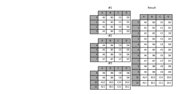
df1 = pd.DataFrame({'A': ['A0', 'A1', 'A2', 'A3'],
                    'B': ['B0', 'B1', 'B2', 'B3'],
                    'C': ['C0', 'C1', 'C2', 'C3'],
                    'D': ['D0', 'D1', 'D2', 'D3']},
index=[0, 1, 2, 3])
|
A |
B |
C |
D |
| 0 |
A0 |
B0 |
C0 |
D0 |
| 1 |
A1 |
B1 |
C1 |
D1 |
| 2 |
A2 |
B2 |
C2 |
D2 |
| 3 |
A3 |
B3 |
C3 |
D3 |
df2 = pd.DataFrame({'A': ['A4', 'A5', 'A6', 'A7'],
                    'B': ['B4', 'B5', 'B6', 'B7'],
                    'C': ['C4', 'C5', 'C6', 'C7'],
                    'D': ['D4', 'D5', 'D6', 'D7']},
index=[4, 5, 6, 7])
|
A |
B |
C |
D |
| 4 |
A4 |
B4 |
C4 |
D4 |
| 5 |
A5 |
B5 |
C5 |
D5 |
| 6 |
A6 |
B6 |
C6 |
D6 |
| 7 |
A7 |
B7 |
C7 |
D7 |
df3 = pd.DataFrame({'A': ['A8', 'A9', 'A10', 'A11'],
                    'B': ['B8', 'B9', 'B10', 'B11'],
                    'C': ['C8', 'C9', 'C10', 'C11'],
                    'D': ['D8', 'D9', 'D10', 'D11']},
index=[8, 9, 10, 11])
|
A |
B |
C |
D |
| 8 |
A8 |
B8 |
C8 |
D8 |
| 9 |
A9 |
B9 |
C9 |
D9 |
| 10 |
A10 |
B10 |
C10 |
D10 |
| 11 |
A11 |
B11 |
C11 |
D11 |
|
A |
B |
C |
D |
| 0 |
A0 |
B0 |
C0 |
D0 |
| 1 |
A1 |
B1 |
C1 |
D1 |
| 2 |
A2 |
B2 |
C2 |
D2 |
| 3 |
A3 |
B3 |
C3 |
D3 |
| 4 |
A4 |
B4 |
C4 |
D4 |
| 5 |
A5 |
B5 |
C5 |
D5 |
| 6 |
A6 |
B6 |
C6 |
D6 |
| 7 |
A7 |
B7 |
C7 |
D7 |
| 8 |
A8 |
B8 |
C8 |
D8 |
| 9 |
A9 |
B9 |
C9 |
D9 |
| 10 |
A10 |
B10 |
C10 |
D10 |
| 11 |
A11 |
B11 |
C11 |
D11 |
# Creating a dataframe from a dictionary
raw_data = {
'Employee ID': ['1', '2', '3', '4', '5'],
'first name': ['Diana', 'Cynthia', 'Shep', 'Ryan', 'Allen'],
'last name': ['Bouchard', 'Ali', 'Rob', 'Mitch', 'Steve']}
df_Engineering_dept = pd.DataFrame(raw_data, columns = ['Employee ID', 'first name', 'last name'])
df_Engineering_dept
|
Employee ID |
first name |
last name |
| 0 |
1 |
Diana |
Bouchard |
| 1 |
2 |
Cynthia |
Ali |
| 2 |
3 |
Shep |
Rob |
| 3 |
4 |
Ryan |
Mitch |
| 4 |
5 |
Allen |
Steve |
raw_data = {
        'Employee ID': ['6', '7', '8', '9', '10'],
        'first name': ['Bill', 'Dina', 'Sarah', 'Heather', 'Holly'],
        'last name': ['Christian', 'Mo', 'Steve', 'Bob', 'Michelle']}
df_Finance_dept = pd.DataFrame(raw_data, columns = ['Employee ID', 'first name', 'last name'])
df_Finance_dept
|
Employee ID |
first name |
last name |
| 0 |
6 |
Bill |
Christian |
| 1 |
7 |
Dina |
Mo |
| 2 |
8 |
Sarah |
Steve |
| 3 |
9 |
Heather |
Bob |
| 4 |
10 |
Holly |
Michelle |
raw_data = {
        'Employee ID': ['1', '2', '3', '4', '5', '7', '8', '9', '10'],
        'Salary [$/hour]': [25, 35, 45, 48, 49, 32, 33, 34, 23]}
df_salary = pd.DataFrame(raw_data, columns = ['Employee ID','Salary [$/hour]'])
df_salary
|
Employee ID |
Salary [$/hour] |
| 0 |
1 |
25 |
| 1 |
2 |
35 |
| 2 |
3 |
45 |
| 3 |
4 |
48 |
| 4 |
5 |
49 |
| 5 |
7 |
32 |
| 6 |
8 |
33 |
| 7 |
9 |
34 |
| 8 |
10 |
23 |
df_all = pd.concat([df_Engineering_dept,df_Finance_dept])
|
Employee ID |
first name |
last name |
| 0 |
1 |
Diana |
Bouchard |
| 1 |
2 |
Cynthia |
Ali |
| 2 |
3 |
Shep |
Rob |
| 3 |
4 |
Ryan |
Mitch |
| 4 |
5 |
Allen |
Steve |
| 0 |
6 |
Bill |
Christian |
| 1 |
7 |
Dina |
Mo |
| 2 |
8 |
Sarah |
Steve |
| 3 |
9 |
Heather |
Bob |
| 4 |
10 |
Holly |
Michelle |
# 머지의 파라미터 left df, right dfm on='공통요소' ,how= left or right 정해진 테이터는 전부 표시
pd.merge(df_all,df_salary, on="Employee ID",how='left')
|
Employee ID |
first name |
last name |
Salary [$/hour] |
| 0 |
1 |
Diana |
Bouchard |
25.0 |
| 1 |
2 |
Cynthia |
Ali |
35.0 |
| 2 |
3 |
Shep |
Rob |
45.0 |
| 3 |
4 |
Ryan |
Mitch |
48.0 |
| 4 |
5 |
Allen |
Steve |
49.0 |
| 5 |
6 |
Bill |
Christian |
NaN |
| 6 |
7 |
Dina |
Mo |
32.0 |
| 7 |
8 |
Sarah |
Steve |
33.0 |
| 8 |
9 |
Heather |
Bob |
34.0 |
| 9 |
10 |
Holly |
Michelle |
23.0 |
댓글남기기